Tuesday, July 11, 2017

反向传播算法

反向传播算法backpropagation

反向传播算法是用来求代价函数C对权重w和偏置b的偏导数的,有了这个偏导数,随机梯度下降算法才可以应用在深度神经网络的学习中。偏导数其实就代表改变本身对代价函数的影响的大小。
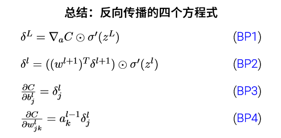
𝜹是代价函数C对节点的偏导数,计算出𝜹后,就可以根据3,4式来计算代价函数C对权重和偏置的偏导数。而𝜹是通过从后向前反向一步一步迭代计算的(公式2),所以,要首先计算输出层没一个节点的𝜹(公式1)。

a是激活值,𝝈是激励函数,w是l层的权重矩阵,b是偏置向量。其中,中间量z是l层的带权输入

在算式BP1中,∇C是代价函数对激活值a的偏导数,可以看到代价函数对激活值a的改变速度。当代价函数C为二次代价函数时,
∇C就是:a-y, 此时BP1就成为:
𝝈'(z)是𝝈对z的导数,表示z处激活函数的变化速率。


实现方法:
def sigmoid(z):
     return 1.0/(1.0+np.exp(-z))

def sigmoid_prime(z):
    return sigmoid(z)*(1-sigmoid(z))

def delta(z, a, y):
    return (a-y) * sigmoid_prime(z)


def backprop(self, x, y):
使用反向传播算法计算𝛁b 和𝛁w
     """Return a tuple ``(nabla_b, nabla_w)`` representing the
gradient for the cost function C_x. ``nabla_b`` and
``nabla_w`` are layer-by-layer lists of numpy arrays, similar
to ``self.biases`` and ``self.weights``."""
nabla_b = [np.zeros(b.shape) for b in self.biases]
nabla_w = [np.zeros(w.shape) for w in self.weights]
# feedforward
activation = x
#用来保存激活值
activations = [x] # list to store all the activations, layer by layer
#用来保存带权输入
zs = [] # list to store all the z vectors, layer by layer
for b, w in zip(self.biases, self.weights):
   
    z = np.dot(w, activation)+b #计算带权输入z
      zs.append(z)
    activation = sigmoid(z)  #计算激活值
    activations.append(activation)
# backward pass
def delta(z, a, y):
# return (a-y) * sigmoid_prime(z)
# 计算BP1
delta = (self.cost).delta(zs[-1], activations[-1], y)
# 计算BP3
nabla_b[-1] = delta
#计算BP4
nabla_w[-1] = np.dot(delta, activations[-2].transpose())
# Note that the variable l in the loop below is used a little
# differently to the notation in Chapter 2 of the book. Here,
# l = 1 means the last layer of neurons, l = 2 is the
# second-last layer, and so on. It's a renumbering of the
# scheme in the book, used here to take advantage of the fact
# that Python can use negative indices in lists.
for l in xrange(2, self.num_layers):
    z = zs[-l]
    sp = sigmoid_prime(z)
    # 计算BP2
    delta = np.dot(self.weights[-l+1].transpose(), delta) * sp
    # 计算BP3
    nabla_b[-l] = delta
    # 计算BP4
    nabla_w[-l] = np.dot(delta, activations[-l-1].transpose())
return (nabla_b, nabla_w)


Monday, July 3, 2017

基于神经网络实现的图像压缩

https://research.googleblog.com/2016/09/image-compression-with-neural-networks.html

在网络中,数据压缩无处不在。在线观看的视频,分享的图片,听到的音乐,甚至现在阅读的博客,压缩技术让你可以快速和高效的分享内容,如果没有压缩技术,将要话费大量的时间和带宽。
在"Full Resolution Image Compression with Recurrent Neural Networks",中,我们使用神经网络扩展了以前在“Variable Rate Image Compression with Recurrent Neural Networks”使用的数据压缩方法,探索了机器学习是否可以提供一个更好的方法,就像他在图像识别和文字概括方面的表现。进一步,我们分享了我们的压缩模型,通过tenforflow, 你可以使用它来压缩自己的图像。
我们引入了一个新的Gated Recurrent Unit的变种,叫做Residual Gated Recurrent Unit (Residual GRU). 我们的Residual GRU是GRU和residual connect的结合,residual connect是在"Deep Residual Learning for Image Recognition"中介绍的,对于给定的压缩率,他可以获得很好的图像质量。与现在的基于DCT的压缩算法不同,我们训练2套神经网络,一套编码,一套解码。
 我们的系统以迭代的方式工作,逐步精细化重建图像,编码器和解码器都是用Residual GRU,附加信息可以从一个迭代向下一次迭代传递。每一次迭代生成一些新的Bit,可以用来提高重建图像质量。概念上,这个网络的工作方式是:
1. 初始残差,R[0]对应于原始图像I,R[0]=I
2. 设置i=1,为第一次迭代
3. 迭代[i]把R[i-1]作为输入,编码和比特化,生成压缩后的码流B[i]
4. 迭代[i]把压缩后的码流B[i]解码,生成重建图像P[i]
5. 计算迭代[i]的残差R[i]=I-P[i]
6. 设置i=i+1,跳转到第三步
残差R[i]代表当前的迭代后,生成图像与原图像有多少差异,R[i]作为输入,交给下一次迭代,目标是消除压缩误差。此时,码率B[1]到B[N]的级联就可以代表压缩图像。N越大,压缩的图像质量就越好。
为了理解他是如何工作,考虑下面的例子。

左边是原始图像,中间是第一次迭代生成的重建图像,右边是残差。

左图是第二次迭代的输入,中间是第二次迭代生成的重建图像,右边是第二次残差。
一个明显的问题是,第二次迭代,为什么可以从残差输入R[1]中,重建出高质量的重建图像P[2]呢?答案是,模型中使用的RNN模型有记忆功能,他在每一次迭代中都保存了信息用于下一次的迭代。在第一次迭代中,他从原始的图像中学习到了一些东西,用来与R[1]一起,从B[2]中生成更好的重建图像P[2]。
在每一次迭代中,网络都得到更多的关于残差的信息,
At each further iteration, the network gains more information about the errors introduced by compression (which is captured by the residual image). If it can use that information to predict the residuals even a little bit, the result is a better reconstruction. Our models are able to make use of the extra bits up to a point. We see diminishing returns, and at some point the representational power of the network is exhausted.


Sunday, July 2, 2017

BinaryConnect:二进制加权训练深层神经网络

BinaryConnect:二进制加权训练深层神经网络
BinaryConnect: TrainingDeepNeuralNetworkswith binaryweightsduringpropagations
MatthieuCourbariaux
´ Ecole Polytechnique de Montr´eal matthieu.courbariaux@polymtl.ca
YoshuaBengio Universit´e de Montr´eal, CIFAR Senior Fellow yoshua.bengio@gmail.com
Jean-PierreDavid
´ Ecole Polytechnique de Montr´eal jean-pierre.david@polymtl.ca


摘要
深层神经网络(DNN)已经在广泛的任务中取得了先进的成果,在大训练集和大量模型的帮助下,得到了最好的结果。在过去,GPU使这些突破成为可能,因为其拥有更高的计算速度的。今后,在训练和测试时,尤其是低功耗设备的消费类应用中,更快的计算很可能是能否取得进一步的进展的关键因素。因此,人们在研究开发深度学习(DL)专用硬件方面有很大兴趣。BinaryConnect,二进制的权重,即,权值被限制到只有两个可能值(例如-1或1),可以给DL带来巨大的好处,因为许多乘法累加操作被简化为加法操作,同时也能节省功耗。我们所说的BinaryConnect,其在于在向前和向后的传播训练DNN中使用二进制权重,同时保持在该梯度中累积的存储权重的精度。类似于dropout操作,BinaryConnect是一种规则化方法,使用这种方法,我们可以获得同等结果,在训练集对置换不变MNIST,CIFAR-10和SVHN中。
引言
深神经网络(DNN)已经在各方面推进了前沿技术的发展,尤其是在语音识别[1,2]和计算机视觉,特别是目标识别 [3,4 ]。最近,深度学习在自然语言处理作出了重要的进展,尤其是统计机器翻译[5,6,7]。有趣的是,取得该重大进展的关键因素之一是图形处理单元(GPU)的出现,速度提高10到30量级,从[8],以及类似的具有分布式训练的改进[9,10]。事实上,近几年的重大突破得益于能够使用大数据训练大模型的能力。如今,研究人员和开发人员在设计新的深度学习算法和应用时,经常发现自己被计算能力所限制。再加上,把深度学习系统应用于低功耗设备的需求,都大大增加了研究和开发深度网络[11,12,13]专用硬件的兴趣。
训练和应用深度网络所需要的大量计算是:由实值激活和实值权重的乘法(在反向传播算法的识别或正向传播相)或梯度(在向后传播相位反向传播算法的)。本文提出了称为BinaryConnect一种方法来降低这种乘法的运算量:强制在前向和反向运算中使用binary权值(只有2个数,1和0)。我们在训练集对置换不变MNIST,CIFAR-10和SVHN中取得了很好的结果

我们的工作之所以可行,源于两个原因
1,在累加和平均大量随机梯度时,足够的精度是必要的,但是噪音权重(以及我们可以查看到离散少数值作为噪音的一种形式,尤其是如果我们做这种离散随机)适用于随机梯度下降算法(SGD),他是深度学习的主要优化算法。 SGD在探索参数空间的时候,通过使用小的和噪音的方法,每个权重都是累积的随机梯度的平均值。因此,要保持足够的精度。乍一看,对高精度的追求绝对是非常重要的。 [14]和[15]表明,随机或随机的舍入可用于提供无偏离散化。 [14]已经表明,SGD要求权重值至少有6至8个比特的精度,[16]表示成功训练DNNs需要12位动态定点计算。此外,脑突触的估计精度为6到12比特[17]。
2.噪声权重实际提供功能是正则化,如前所述,通过使用变量噪声[18],dropout[19,20]和DropConnect [21]向激励或权重增加噪声。例如,DropConnect [21],比较类似于BinaryConnect,是一种非常有效的正则化方法,它随机的把一半的权值用0来代替。所有这些以前的工作都表明,只有权值的期望值需要具有高精度,并且,噪音实际上是有益的。
这篇文章的主要贡献有以下几种。
•我们介绍BinaryConnect,在DNN中使用,在向前和向后的传播中使用。
•我们证明了BinaryConnect是一个正则化方法,我们在MNIST,CIFAR-10和SVHN(第3节)取得了很好的效果。

•我们为BinaryConnect编写了.的代码

2 BinaryConnect

在本节中,我们给出BinaryConnect的更详细的描述,包括如何选择这两个值,如何离散化,如何训练和推论。
2.1 +1和-1
一个DNN的应用只要包含卷积和矩阵乘法。于是,关键的运算就是乘加运算。神经元把权值乘以输入,再加在一起。
BinaryConnect在传播的过程中,把权值限制为+1或-1两个值。于是,乘加运算简化为加法。

2.2 确定的和随机的二值化
二值化操作把实值权值变成2个可能值。一个最直接的二值化方法就是取符号
Wb = +1 w>=0; -1 w<0
Wb是实值权值w的二值化。虽然这是一个确定的操作,但是因为隐藏层节点很多,这么多的值上的平均化可以弥补信息的损失。
另一种方法可能更好,平均值更加的正确,就是随机二值化方法
Wb = +1 概率p=Q(w); =-1 概率1-q
其中Q是hard sigmoid函数:
Q(x) = clip((x+1)/2,0,1) = max(0,min(1,(x+1)/2))
我们使用hard sigmoid而不是sigmoid,因为hard sigmoid更容易计算,而且从实验结果看也不错。
2.3 传播和更新
让我们考虑随机梯度下降更新算法中的不同阶段
1. 给定DNN输入,逐层计算单元的活动直到顶层,顶层为DNN的输出层,这一步为前向传播
2. 给定DNN输出,计算训练目标的梯度,也就是每一层的行为,从顶层向下直到第一个隐藏层,这一步叫后向传播
3. 计算梯度,使用新的梯度和旧的值,更新权值,这一步叫权值更新

算法:
BinaryConnect的SGD训练方法:C为cost函数,binary()为二值化方法,clip()为clip权值的函数,L是层数
需求:输入,目标,上一次的权值Wt-1和偏移Bt-1,学习速度l
保证:更新权值Wt和偏移Bt
1. 前向传播
Wb=binary(Wt-1)
对每一层k,前向计算各个节点的输出Ak
2. 后向传播
初始化输出层的激励梯度,使用梯度和权值Wb,反向计算上一层的梯度
3. 参数更新
根据激励梯度和激励,计算权值梯度和偏移梯度,更新权值和偏移


BinaryConnect的关键一点是binary方法只有在前向和后向传播的时候使用,在参数更新的时候不使用,此时仍然使用原来的实值权值。SGD算法要求在更新参数的时候保持精度的权值。通过梯度下降而取得的参数的改变是非常小的,SGD对大量的节点做很小的修改来得到训练目标。一种理解这种算法的方法是假设:在训练结束时,最重要的是权值的符号


Saturday, June 17, 2017

基于RNN的编码率图像压缩

基于RNN的编码率图像压缩
VARIABLE RATE IMAGE COMPRESSION WITH RECURRENT NEURAL NETWORKS
GeorgeToderici,SeanM.O’Malley,SungJinHwang,DamienVincent {gtoderici, smo, sjhwang, damienv}@google.com DavidMinnen,ShumeetBaluja,MicheleCovell&RahulSukthankar 

介绍
互联网上有很多的数据传输是来自于移动设备的驱动,这些移动设备的屏幕较小,带宽不大。因此,对于有很多图片的网站,提供传送低解析度,低码率的预览图片可以明显提高网页的响应速度。提供比现有的压缩质量更高的缩略图压缩方法成为了一个研究方向,带宽的节省可以提高移动设备用户的体验。为此,我们提供了一个可变码率图像压缩的框架,一个全新的架构,基于卷积和反卷积的LSTM网络。我们的方法,解决了autoencoder不能和现有的图像压缩算法抗衡的问题:(1)我们的网络只依赖于一次训练(与图像无关),不用考虑图像的大小和需要的压缩率。(2)我们的网络是渐进的,这意味着更多的Bit被传送,就可以得到更好的图像质量。(3)这个架构和已有的标准的有目的的autoencoder一样有效。在基于32x32的缩略图的测试中,我们的基于LSTM的方法比已有的JPEG,WebP标准更好,压缩文件大小可以降低10%。

  1. 介绍

多年来,图像压缩的任务被很多研究人员和团队研究,如联合图像专家组,他们设计的无处不在的JPEG和JPEG 2000(ISO / IEC 15444-1)的图像格式。最近,WebP算法,进一步提高图像压缩率(谷歌,2015年),特别是对于那些在最近几年变得越来越普遍的高分辨率图像。所有这些努力都是从实证的角度出发:人类专家设计的各种探索,以减少需要被保留的信息,然后找到转换这种信息的。这项工作几乎全部集中在大size图像的压缩,低分辨率的缩略图像通常被忽略(甚至伤害,例如,通过要求在文件头更多的数据)。

标准的图像压缩算法往往做出图像Size的假设。例如,我们通常认为从高分辨率自然图像中的一块图像,包含大量的冗余信息。事实上,分辨率越高的图像,他的小块图像越有可能包含更多的低频信息。这一事实被大多数图像编解码器使用,正因为如此,这些编解码器往往是在压缩的高分辨率图像非常有效。但是,创建高分辨率自然图像的缩略图时,这样的假设是不成立的,因为缩略图中小块区域包含难以压缩的高频信息。
大量压缩缩略图(32x32)是一个重要的应用,在减少硬盘的存储量和更好的使用带宽方面。网页的预览图像,相片集,搜索引擎和大量其他的应用都要传输缩略图。在缩略图压缩方面的任何改进都可以提高应用的体验。
最近,神经网络已经成为了推进已有算法的工具。例如,在图像识别和对象检测,当前状态的最先进的算法都是基于神经网络。这是很自然要问,如果我们也可以使用这个功能强大的类的方法来进一步提高图像压缩的任务,特别是对我们不都经过精心设计,手工调整压缩方法的图像尺寸。
如果我们把图像压缩算法看作是一个包含瓶颈的分析综合系统,这样我们就可以训练神经网络开发出压缩的表达。大量的已有的工作室在小图像上做的:32x32的CIFAR10。这些工作都被分在autoencoder里面。但是,多数的autoencoder都是在一些硬性的限制下工作的,让他们无法替代普通的图像编码算法。有些限制使得编码率压缩没法实现。输出的图像质量很难保证,很多都是为了特定大小的图像训练的,可以在特定大小的图像上找出冗余信息。
我们探索的几种神经网络驱动的编码算法,与已有的图像压缩算法有相似的灵活性。为了达到这些灵活性,我们的算法必须符合这些要求:1)压缩率可以预先设定。2)根据图像内容的复杂简单程度分配码率。3)模型是从大量已有的图像中学习的,这样可以应付真实的图像
  1. 相关工作
使用前向神经网络实现图像压缩的概念已经有一段时间了(Jiang 1999)。在这篇文章里,神经网络可以辅助甚至完全的替代很多工作,他是作为一个与传统图像压缩并行的工作:可以学习到更加有效的频域转换算法,更加有效的量化技术,提高预测编码。
最近,autoencoder技术 (Hinton & Salakhutdinov, 2006) 已经在端到端的压缩中可以使用。一个典型的autoencoder有3个组成:1)编码器把一个固定维度的图像编码成 2)一个瓶颈,可以理解为压缩后的数据,这些数据被 3)解码器还原成原始图像。这三个部分合在一起进行端到端的训练,使用的时候分别使用。
瓶颈通常是一个简单的平面神经网络层,通过调整这一层的节点数目,可以控制压缩率和压缩图像质量。这种autoencoder,把瓶颈编码成简单bit向量是有效的 (Krizhevsky & Hinton, 2011)。在基于神经网络的分类任务中,不断地卷积和池化可以下采样图像,输出是一些简单的结点。在autoencoder的解码器中,网络必须反向处理,把这些简单的结点转化成大的图像。当这种上采样图像是spatially-aware的,类似于反向卷积,一般被叫做解卷积。 (Long et al., 2014).
LSTM网络是一种RNN网络,在语音识别和机器翻译方面已经被证实非常有效。很多LSTM的扩展模型可以包含显示的空间信息的操作,衍生出各种卷积LSTM,他们可以更好是适用于图像处理。
我们尝试了这种卷积LSTM,同时尝试递归的架构,把一个autoencoder的残差输出作为另一个autoencoder的输入。

  1. 可变码率压缩结构
我们通过描述一个一般的基于神经网络的压缩架构,然后再讨论这一架构的多个实例的细节入手。每个小节介绍了不同的架构,建立在以前的模式,提高了压缩效果。

对于每个结构,我们将讨论一个函数E,它接受一个图像块作为输入,并产生一个编码表示。这种表示通过二值化函数B,(B也有同样的结构,在3.2节中进行讨论)最后,对于每个结构,我们还考虑一个解码器功能D,这把由B中产生的二进制表示,重构输出图像块。连在一起,这三种模块形成自动编码器x = D(B(E(X))),这是对于所有的压缩网络的基本构建块。
对于所有的结构中,偏移和缩放被施加到8位RGB输入图像,得到-0.9和0.9之间的范围的值。这个范围与tanh的值相兼容。
    1. 图像压缩框架

我们使用共享相同的架构设计:编码器,进行量化和解码器。此外,我们的框架是支持可变压缩率,而且不需要重新培训,也不需要存储同一图像的多个编码输出。
为了能够传递增量信息,设计时应考虑到一个事实,即图像解码将是渐进的。有了这个设计目标,我们可以考虑一种架构:构建在解码器获得附加信息,减少残差编码误差。
形式上,我们链接多个用于残差编码的autoencoder:
Ft(rt−1) = Dt(B(Et(rt−1))).
在前向网络(3.3和3.5节)中,这个链接是显性的。在使用LSTM的网络(3.4和3.6节)中,它是隐性的。我们假设r0是原始图像,Ft没有记忆,此时我们只想预测残差本身。此时,图像的重建是靠把所有的残差合在一起,没一个autoencoder的loss是原始残差和预测的残差的差
rt = Ft(rt−1)−rt−1.
另一方面,在LSTM网络中,LSTM有记忆,会保留状态,我们在每一次autoencoder中,使用它来预测原始图像,因此,loss是原始图像和预测的差
rt = Ft(rt−1)−r0.
相同的是,rt被转化成||rt||2

    1. bit表达
在我们的网络中使用的bit表达方法是首先由 Williams (1992)提出的,类似于 Krizhevsky & Hinton (2011) and Courbariaux et al. (2015). 这种方法有3个有点:(1)这种方法是为了传输图像而设计的序列化和反序列化方法。(2)通过简单的显示bit数就可以控制压缩率。(3)bit的瓶颈可以帮助网络学习来提高表达效率,而普通的浮点层,可能包含冗余的bit

二值化处理由两个部分组成。第一部分包括产生所需数量的输出,输出值在连续区间[-1,1](等于输出的期望的数量)。第二部分包括取这个实值表示作为输入,并产生离散输出,在集合{-1,1}。
在二值化过程的第一步中,我们使用具有tanh激活的全连接层。对于第二部分,使用 Raiko et al. (2015),的方法。一个可能的值B(X)x∈[-1,1]被定义为
b(x) = x + e, e ∈{−1,1},
e是量化噪音。我们使用随机量化提供的正规化来做后向传播的梯度。 We will use the regularization provided by the randomized quantization to allow us to cleanly backpropagate gradients through this binarization layer.
这样,全部的二值化编码过程就是:
B (x) = b(tanh(Wx + b)).
W和b是权值和偏移,但是是二值化后的。在我们的模型中,前向计算中都是使用这个公式。在后向传播中,我们使用期望的导数。(Raiko et al., 2015). 因为B(x)的期望还是x,因此,导数通过二值化层的时候没有变化
对于特定的输入图像,为了产生一个固定的表达,一旦网络被训练好了,只有最有可能的输出值b(x)需要被考虑,b可以被binf替代:
binf(x)=-1 if x<0; +1 other
压缩率由每一步生成的bit数决定,它对应到权值W的个数乘以autoencoder重复的次数。
    1. 前向全链接残差编码
在我们各种编码率压缩算法中,最简单的是全链接网络,E,D由全链接层组成。我们设置每一层的节点数为512,激励函数为tanh。
没一次递归,可以有不同的E和D,因为每一次递归,需要编码的残差图像都有不同统计分布。因此,我们考虑2中方式:第一种方式,每一次递归分享同一组权值,第二种方式,每一次递归训练自己的专有的权值。

    1. 基于LSTM的压缩

在这种架构中,我们探索利用LSTM模型的编码器和解码器。特别地,E和D都包括层叠LSTM层。
继萨伦巴等人提出的LSTM公式和符号(Zarembaetal.(2014),),我们使用上标以指示层号,下标表示time step。hlt表示time step为t的第l个隐藏层。定义Tln为仿射变换
Tln(x)=wlx+bl
定义⊙为点乘,h0t为time step 为t时第0层的输入。
使用这些符号,这个LSTM架构可以表示为

In these equations, sigm and tanh are applied element-wise. This alternate formulation of LSTM is useful because it reduces the numbers of separate operations needed to evaluate one step, which allows for an efficient implementation on GPU.
用于编码器中,我们使用一个全连接层,然后堆叠两个LSTM层。该解码器具有相反的结构:两个堆叠LSTM层,然后一个全连接层,使用tanh激励,用其预测RGB值(我们省略图中的这个层以减少混乱)。在实验中使用的确切结构在图2中(减去RGB转换)中给出。
    1. 前向卷积反卷积残差编码

第3.3节给出的全连接的残差autoencoder。我们扩展这个结构,把全链接造作替换成卷积操作,解码器的最后一层是一个1x1的卷积层,有3个filter,把解码输出转换成RGB。我们描绘在图3这个架构(减去RGB转换)。
反卷积操作定义为卷积的转置,


    1. 卷积反卷积LSTM压缩
最后的结构把卷积反卷积和LSTM结合在一起。我们把方程8中的Tl4n操作用卷积加偏移来替换,这样,卷积LSTM的变换函数就变成了
T的上标l对应的是深度,也就是输出的feature的index,第二个卷积项代表卷积LSTM的recurrent关系,所以他的输入和输出必须有相同的大小。因此,如果一个卷积LSTM的stride大于2,那它只能用于第一个卷积操作项,第二项的stride必须是1。最后,把卷积编码器中的第二和第三个卷积层替换成卷积LSTM层。
对于解码器,不能把所有的卷积都直接替换成反卷积,因为反卷积的输入和输出通常是有不同的维度。因此,定义反卷积LSTM为:
下标c是卷积层的权值,下标d是反卷积层的权值。
在解码器中,第二层和第三层使用反卷积LSTM层替换

    1. 动态bit分配

对于这里给出的非卷积方法,很自然通过允许不同数量的编码器的迭代以分配不同数量的每个色块的比特。这可以通过目标质量度量(例如,PSNR)来确定。虽然不自然,在卷积方法的情况下,类似的方法也可以采用。输入图像需要被分成补丁,和每个补丁独立地处理,从而允许不同数量的每个区域的比特。然而,这种方法将在本文的最后讨论的缺点。

  1. 实验和分析
    1. 训练
为了训练各种神经网络的配置,我们使用Adam算法。 Kingma & Ba (2014)。 训练速度为{0.1,0.3,0.5,0.8,1}。
对于卷积网络,输入为32x32的块,下采样到8x8,每个像素用2个Bit表示,这样每个32x32的块编码成16个byte。
    1. 评估
使用SSIM评估图像质量,1代表最好,0代表最差
    1. 32x32比较
    2. 分析

  1. 结论和将来的工作
Whileourcurrentapproachgivesfavorableresultsversusmoderncodecsonsmallimages,codecsthat include an entropy coder element tend to improve (in a bits-per-pixel sense) with greater resolution, meaning that by choosing an arbitrarily large test image it is always possible to defeat an approach like that described in this work. Therefore, an obvious need is to extend the current work to function on arbitrarily large images, taking advantage of spatial redundancy in images in a manner similar to entropy coding. Although we presented a solution for dynamic bit assignment in the convolutional case, it is not a fully satisfactory solution as it has the potential to introduce encoding artifacts at patch boundaries. Another topic for future work is determining a dynamic bit assignment algorithm that is compatible with the convolutional methods we present, while not creating such artifacts. The algorithms that we present may also be extended to work on video, which we believe to be the next grand challenge for neural network-based compression.

Sunday, January 15, 2017

study: openCL programming

memory in GPU.

  • global memory: all work-item can access. transit between CPU and GPU
  • constant memory
  • local memory: faster, in workgroup 
  • private memory
relation between OpenCL memory model with AMD HD6970

Synchronize :
  • in kernel: barrier() (marker) barrier(CLK_LOCAL_MEM_FENCE)
  • between CPU and GPU: CL_TRUE, clfinish()
  • event: clWaitForEvent()
event.getProfilingInfo() for debug
event.clsetEventCallback() callback host function when the event happen

Native Kernel: execute in host. unboxing

fence operation: make sure memory read/write should be done
Atomic operation: atomic_add() atomix_xchg()

for constant data, we can use clDeviceInfo() to get the size and number of divice: CL_DEVICE_MAX_CONSTANT_ARGS CL_DEVICE_MAX_CONSTANT_BUFFER_SIZE

One wavefront execute on all work-time, branch in wavefront have very poor efficient, see below:

memory access: channel and bank. 
one wavefront should try to access on channel and bank 64KB, it is most efficient.

memory access: channel and bank. 
one wavefront should try to access on channel and bank 64KB, it is most efficient. 

Profiler:
AMD: 
  • Accelerated Parallel Processing Profiler
  • Accelerated Parallel Processing Kernel Analyzer
  • gDEBugget
  • clGetEventProfileingInfo(): get event time infomation

Tuesday, January 10, 2017

study: GPU programming CUDA OpenCL

GPU and host memories are typically disjoint, requiring explicit (or implicit, depending on the development platform) data transfer between the two. 

CUDACompute Unified Device Architecture. provides two sets of APIs (a low, and a higher-level one), and it is available freely for Windows, Mac OS X, and Linux operating systems. Although it can be considered too verbose, for example requiring explicit memory transfers between the host and the GPU, it is the basis for the implementation of higher-level third-party APIs and libraries, as explained below. 
OpenCLOpen Computing Language. supported by both Nvidia and AMD. It is the primary development platform for AMD GPUs. OpenCL’s programming model matches closely the one offered by CUDA.

CUDA:
Support heterogeneous computation where applications use both the CPU and GPU. Serial portions of applications are run on the CPU, and parallel portions are offloaded to the GPU. As such, CUDA can be incrementally applied to existing applications. The CPU and GPU are treated as separate devices that have their own memory spaces. This configuration also allows simultaneous computation on the CPU and GPU without contention for memory resources.

In order to properly utilize a GPU, the program must be decomposed into a large number of threads that can run concurrently. GPU schedulers can execute these threads with minimum switching overhead and under a variety of configurations based on the available device capabilities. 

Threads are organized in a hierarchy of two levels, as shown in Figure 6.3. At the lower level, threads are organized in blocks that can be of one, two or three dimensions. Blocks are then organized in grids of one, two, or three dimensions. The sizes of the blocks and grids are limited by the capabilities of the target device.
In every block, it is a kernel. A same function run in all kernel at same time. 
hello<<<2,10>>> ()
mean function hello() will run 20 time same-time, one time in one kernel.
an example: 
__global__ void hello()
{
   printf("hello world\n");
}
int main()
{
   hello<<<1,10>>>();
   cudaDeviceSynchronize();
}
it will display "hello world" 10time, cudaDeviceSynchronize() is a barrier. waiting for the execute result. function hello() is execute on devices, although it called by host. 
Each kernel function has two dimension: grid and block. this mean function has grid index and block index.

What's Warp:
In GPU, same kernel instruction is executing in different process unit (SP: Stream processor). This collection of SP under same controller is SM: Streaming Multiprocessor.
One GPU contains multiple SM, each SM run each own kernel.  In nVidia, one SP == CUDA core.  Nvidia calls this execution model Single-Instruction, Multiple Threads (SIMT).
I feel One SM is One block. 
Warp: The threads in a block do not run concurrently, though. Instead they are executed in groups called warps

Threads in a warp may execute as one, but they operate on different data. So, what happens if the result of a conditional operation leads them to different paths? The answer is that all the divergent paths are evaluated (if threads branch into them) in sequence until the paths merge again. The threads that do not follow the path currently being executed are stalled.
see the example:


Monday, January 9, 2017

study: OpenCL Intel GPU: install SDK


  • I download opencl sdk for intel GPU from https://software.intel.com/en-us/intel-opencl/download it ask my email to register, then, star download ntel_sdk_for_opencl_setup_6.3.0.1904.exe (276 MB)
  • click the exe file, it will install intel sdk for opencl in folder: intel\opencl SDK\6.3 after install, it require restart computer. the folder is about 500M, but there is no sample file.
  • I think I can copy sample file from amd opencl package. this package is big, about 522M, it contain: 
    • bolt
    • c++AMP
    • opencl
    • opencv
  • in eopncl, we click OpenCL2.0SamplesVS13, this solution includes lots of project, we select HelloWorld to compile, there are error. obviously, the error is come from the proejct still don't know the position of opencl header file and lib. then we need add AMDAPPSDKROOT into environment variables, we set it equal to C:\Program Files (x86)\Intel\OpenCL SDK\6.3
  • then, recompile the project, it success. we can run it. it display "Passed". but, not all project works. some of them miss CLUtil.hpp file
  • after install, we can found in the vs, there is a new menu item: code-builder . it is for opencl development. https://software.intel.com/en-us/intel-opencl/ there are several video teach you how to use it 

study: Multicore and GPU programming (1)

CPUs employ large on-chip (and sometimes multiple) memory caches, few complex (e.g., pipelined) arithmetic and logical processing units (ALUs), and complex instruction decoding and prediction hardware to avoid stalling while waiting for data to arrive from the main memory.
Instead, GPU designers chose a different path: small on-chip caches with a big collection of simple ALUs capable of parallel operation, since data reuse is typically small for graphics processing and programs are relatively simple. In order to feed the multiple cores on a GPU, designers also dedicated very wide, fast memory buses for fetching data from the GPU’s main memory.
Now it becomes obvious why having CPU and GPU cores share and access the same memory space is an important feature. On principle, this arrangement promises better integration of computing resources and potentially greater performance, but only time will tell.

THE CELL BE PROCESSOR

Cell features a design well ahead of its time: a master-worker, heterogeneous, MIMD machine on a chip.
The hardware was designed for maximum computing efficiency but at the expense of programming ease. The Cell is notorious for being one of the most difficult platforms to program on.

NVIDIA’S KEPLER


The cores in a Kepler GPU are arranged in groups called Streaming Multiprocessors (abbreviated to SMX in Kepler, SM in previous architectures, and SMM in the upcoming Maxwell). Each Kepler SMX contains 192 cores that execute in a SIMD fashion, i.e., they run the same sequence of instructions but on different data. Each SMX can run its own program, though. The total number of SMX blocks is the primary differentiating factor between different chips of the same family. The most powerful chip in the Kepler family is the GTX Titan, with a total of 15 SMXs. One of the SMXs is disabled in order to improve production yields, resulting in a total of 14 · 192 = 2688 cores! The extra SMX is enabled in the version of the chip used in the dual-GPU, GTX Titan Z card, resulting in an astonishing package of 5760 cores! AMD’s dual-GPU offering in the form of the Radeon R9 295X2 card is also brandishing 5632 cores in a shootout that is delighting all high-performance enthusiasts.

AMD’S APUS

What is significant is the unification of the memory spaces of the CPU and GPU cores. This means that there is no communication overhead associated with assigning workload to the GPU cores, nor any delay in getting the results back. This also removes one of the major hassles in GPU programming, which is the explicit (or implicit, based on the middleware available) data transfers that need to take place.
HSA is arguably the way forward, having the capability to assign each task to the computing node most suitable for it, without the penalty of traversing a slow peripheral bus. Sequential tasks are more suitable for the LCU/CPU cores, while data-parallel tasks can take advantage of the high-bandwidth, high-computational throughput of the TCU/GPU cores.


Monday, January 2, 2017

bookmark: H265 vs H264 codec

A Comparison of H.264 and H.265
FunctionH.264H.265
Coding unit16 × 16 macroblock64 × 64, 32 × 32, 16 × 16 coding tree unit
64 × 64, 32 × 32, 16 × 16, 8 × 8 coding unit
Prediction16 × 16, 16 × 8, 8 × 16, 8 × 8, 8 × 4, 4 × 8, 4 × 464 × 64 to 4 × 4, symmetric/asymmetric
Transform size8 × 8, 4 × 432 × 32, 16 × 16, 8 × 8, 4 × 4
TransformDCTDCT, optional DST for 4 × 4
Intraprediction9 modes35 modes
Luma interpolation6-tap filter for 1/2 sample followed by bilinear interpolation for 1/4 sample8-tap filter for 1/2 sample, 7-tap filter for 1/4 sample
Chroma interpolationBilinear interpolation4-tap filter for 1/8 sample
InterpredictionMotion vectorAdvanced motion vector prediction (spatial and temporal)
Entropy codingCABAC, CAVLCCABAC
In-loop filteringDeblockingDeblocking followed by sample-adaptive offset
Parallel processingSlices, slice groupsSlices, tiles, wavefronts
H265 GOP
Different from mpeg4, the B frame can used as referenced or unreferenced.


Unlike H264, H265 GOP could start without IDR frame.An IDR frame is independently coded and frames that follow it in the bitstream will not reference frames prior to it. To implement it, H265 define complex frame: 
  • CRA: clean random access frame: new, independently coded frame that starts at an RAP
  • BLA: broken-link access  frame
  • RASL: random access skipped leading frame
  • RADL:random access decodable leading frame
RASL frames and RADL frames are leading frames because their display order (i.e., encoder output order) precedes the RAP frame even though they appear after the RAP frame in the decoding order.

RDO (High Complexity) When Compared to No RDO
ModeEncoding TimeCompression EfficiencyVideo Quality
VBRLonger (especially for low QP)LowerBetter for every frame (especially for low QP)
CBRLongerNABetter (especially for low QP)